$\newcommand{\E}{\mathbb{E}}$ $\newcommand{\argmax}{\mathrm{argmax}}$ $\newcommand{\Mu}{M}$ $\newcommand{\ba}{\bar{a}}$ $\newcommand{\hx}{\hat{x}}$ $\newcommand{\argmin}{\mathrm{argmin}}$ $\newcommand{\sigmasqr}{\sigma^2}$ This article synthesizes insights from multiple original research papers and both English and Chinese academic sources, with original analysis and derivations by the author.

Todo list

• Translate to Markdown
• Check Equations
• Fix Image & Website References

Preliminary

Understanding the following concepts:

Data Distribution

Markov Process

Normal Distribution

Cross Entropy

Likelihood

Differential Equations

1. Variational Auto Encoders

1.1 VAE and CVAE

Although the title is Diffusion Model, it’s necessary to discuss its ancestor — Variational Auto Encoder. We consider an image generation model containing:

1. Encoder $\mathcal{E}$
2. Decoder $\mathcal{D}$

And it works as follows: For a given input $x$, $\mathcal{E}(x)=(\mu_x,\sigma_x)$, let $z\sim\mathcal{N}(z;\mu_x,\sigma_x)$ be a random sample, apply $\hx=\mathcal{D}(z)$ and traditionally apply reconstruction loss. In this process, we don’t want the variance of the latent variable $z$ to degenerate to 0, and for generation capability we want the distribution of this latent variable to approximate $\mathcal{N}(0,1)$ (so we can directly sample). Therefore, we consider $D_{KL}(\mathcal{N}(\mu,\sigma)\parallel\mathcal{N}(0,1))$:

\[\begin{align*} D_{KL} &= \int \frac{1}{\sqrt{2\pi\sigmasqr}}e^{-\frac{(x-\mu)^2}{2\sigmasqr}}\log \frac{\frac{1}{\sqrt{2\pi\sigmasqr}}e^{-\frac{(x-\mu)^2}{2\sigmasqr}}}{\frac{1}{\sqrt{2\pi}}e^{-\frac{x^2}{2}}}dx \\ &= \int \frac{1}{\sqrt{2\pi\sigmasqr}}e^{-\frac{(x-\mu)^2}{2\sigmasqr}}\log{\frac{1}{\sqrt{\sigmasqr}}e^{\frac{x^2-(x-\mu)^2}{2\sigmasqr}}}dx \\ &= \frac{1}{2}\int \frac{1}{\sqrt{2\pi\sigmasqr}}e^{-\frac{(x-\mu)^2}{2\sigmasqr}}[-\log \sigmasqr+x^2-\frac{(x-\mu)^2}{\sigmasqr}]dx \\ &= \frac{1}{2}(-\log\sigmasqr+\mu^2+\sigmasqr-1) \end{align*}\]

Then we add this as a regularization term in the loss.

Note that the normal distributions in this section are not written in multivariate form, but the principle is the same, because in multivariate case the term under the square root is $|\Sigma|=|\sigma I|=\sigma^n$

For Conditional VAE — Conditional Variational Auto Encoder, one approach is to allow the above loss to have multiple different $\mu$ (classified by category) for control, another approach is to directly use the condition as one of the inputs to the Decoder. This way the latent variable will model other parts, such as details. https://ijdykeman.github.io/ml/2016/12/21/cvae.html

1.2 ELBO

This section will derive the famous Evidence Lower Bound (variational Bayesian inference), because it’s so commonly used. Suppose there is an unknown variable $z\sim p(z|x)$ on the observed $x$, we want to train a $q(z)$ such that $q(z)\approx p(z|x)$. We naturally want to minimize the divergence $D_{KL}[q(z)||p(z|x)]=\int q(z)\log \frac{q(z)}{p(z|x)}$. Expanding the conditional probability and expanding the log, we get $D_{KL}=-\int q(z)\log p(z,x)dz+\int q(z)\log q(z)dx+p(x)\int q(z)dz$. Thus we have $D_{KL}=\E_{z\sim q(z)}[\log q(z)]-\E_{z\sim q(z)}[\log p(z,x)]+p(x)\ge \E_{z\sim q(z)}[\log q(z)]-\E_{z\sim q(z)}[\log p(z,x)]\ge 0$. Therefore we have $\E_{z\sim q(z)}[\log q(z)]\ge\E_{z\sim q(z)}[\log p(z,x)]$.

We define the evidence lower bound as $-\text{ELBO}(q)=\E_{z\sim q(z)}[\log q(z)]-\E_{z\sim q(z)}[\log p(z,x)]$. Actually, through transformation we can obtain $-\text{ELBO}(q)=\E[\log q(z)-\log p(z)]-\E[\log p(x|z)]=D_{KL}[q(z)||p(z)]-\E[\log p(x|z)]$.

1.3 Connection between VAE and ELBO

Consider modeling this problem: we have a data distribution $X$, and each data point $x$ is viewed as sampled from it. We want to train a model $p_\theta(x)$ to fit the data distribution. A natural idea is to use maximum likelihood to maximize $\log p_\theta(x)$. Here we introduce a latent variable $z$, then we have $\log p_\theta(x)=\int \log [p_\theta(x)]q(z|x)dz$. We don’t parameterize first, and continue transforming to get $\int q(z|x)\log [\frac{p(x,z)}{q(z|x)}\frac{q(z|x)}{p(z|x)}]dz=\int q(z|x)\log \frac{p(z)}{q(z|x)}dz+\int q(z|x)\log p(x|z)dz + D_{KL}[q(z|x)||p(z|x)]$.

So our objective is $\mathcal{L}=\E_{z\sim q(z|x)}[\log p(x|z)] -D_{KL}[q(z|x)||p(z)]+D_{KL}[q(z|x)||p(z|x)]$. It’s not hard to see that since $z$ is introduced, it means $q(z|x), p(z|x), p(z)$ will all be arbitrary. Then we can reasonably make the following bound:

$\mathcal{L} \ge \E_{z\sim q(z|x)}[\log p(x|z)] -D_{KL}[q(z|x)||p(z)]$. Then we specify a prior $p(z)=\mathcal{N}(0,I)$, and subsequently use neural networks to model $p(x|z)$ and $q(z|x)$, which gives us the VAE form. We can see that the right side of the final inequality is exactly ELBO. More theoretically speaking, the term $\E_{z\sim q(z|x)}[\log p(x|z)]$ is key. We take the expectation of the log likelihood, our optimization objective is $\argmax_\theta \E_{x\sim X}[\log p_\theta(x)]$. Substituting this term and taking expectation gives $\E_{x\sim X}[\E_{z\sim q(z|x)}\log p(x|z)]=\sum_x\sum_zq(z|x)\log p(x|z)$. The $p(x|z)$ modeled by VAE outputs an image, which can be seen as predicting $\E_{x\sim p(x|z)}[x]$. Therefore we cannot directly estimate this expectation, so we use Monte Carlo methods, which returns to the form equivalent to L2 Loss.

Of course, there’s another way to quickly get the result we want, which is: $\log p(x)=\log \int p(x,z)dz=\log \int \frac{p(x,z)}{p(z)}p(z)dz \ge\int \log[ \frac{p(x,z)}{p(z)}]p(z)dz=\E[\log p(x,z)]-\E[p(z)]=\text{ELBO}$

Then we just need to replace the distribution of $z$ to get similar results as above.

There’s a strange point here: if we really have $D_{KL}[q(z|x)||p(z)]=0$, then the decoder cannot get any information from $z$. However, this objective is also in our optimization goal, which seems contradictory. This is actually the so-called VAE posterior collapse problem. For more detailed introduction, refer to https://blog.csdn.net/wr1997/article/details/115255712. In summary, although ELBO indeed needs this divergence term, it’s very likely to cause the model to fall into a local minimum that it cannot escape from, leading to posterior collapse. That is, optimizing $\E[\log p(x)]$ is indeed optimizing ELBO, but direct optimization will cause falling into local minima.

Here it’s necessary to explain the notation $p$ and $q$ we introduced. You might wonder how they should be defined in a rigorous probability space. My personal understanding is that they can be seen as two probability measures introduced on the standard $\sigma$-algebra, i.e., two probability spaces $<\Omega,\mathcal{F},P>$ and $<\Omega,\mathcal{F},Q>$, but they share the same algebra and domain of random variables.

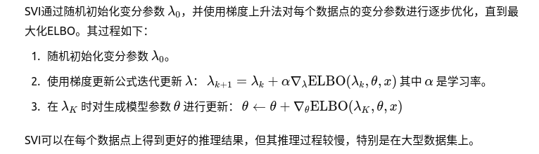
1.4 Stochastic Variational Inference

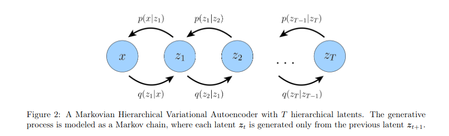
1.5 Hierarchical VAEs

Please refer to the following two papers:

1. Durk P Kingma, Tim Salimans, Rafal Jozefowicz, Xi Chen, Ilya Sutskever, and Max Welling. Improved variational inference with inverse autoregressive flow. Advances in neural information processing systems, 29, 2016.

2. Casper Kaae Sønderby, Tapani Raiko, Lars Maaløe, Søren Kaae Sønderby, and Ole Winther. Ladder variational autoencoders. Advances in neural information processing systems, 29, 2016.

After reading this, I believe your understanding of diffusion is beyond the scope of seeing it as something from outer space.

1.6 VQ-VAEs

We mentioned earlier that VAE suffers from posterior collapse. However, for continuous distribution VAEs, we cannot let them decide the prior distribution by themselves — this would make sampling impossible. But for discrete distributions, it’s easy to fit the prior distribution after model training is complete. This leads to VQ-VAE. There shouldn’t be too many difficulties here, so just read the paper: https://arxiv.org/pdf/1711.00937

2. DDPMs

2.1 Theory

2.1.1 Forward Process

Let the data distribution $q(x^0)$ be gradually transformed by Markov diffusion kernel $T$ into a well-behaved distribution (normal distribution). Define one-step transformation as: $q(x^{t+1})=\int dx^tT(x^{t+1}|x^t;\beta)q(x^t)$, where $\beta$ is the kernel control parameter. We also define $q(x^{t+1}|x^{t})=T(x^{t+1}|x^t;\beta)$, which is obviously Markovian. We have $q(x^{0…T})=q(x^0)\prod_{t=1}^Tq(x^t|x^{t-1})$. There’s also a theorem: if the kernel is Gaussian, then the reverse process is also Gaussian.

2.1.2Reverse Process

We use distribution $p(x^t)$ to represent the model-fitted distribution. We must have $\lim_{T\to \infty} p(x^T)=\mathcal{N}$. Since the reverse process is also Markovian, we have $p(x^{0…T})=p(x^T)\prod_{t=1}^Tp(x^{t-1}|x^t)$, then obviously the integral gives $p(x^0)=\int dx^{1…T}p(x^{0…T})$. What we want is $p(x^0)=q(x^0)$, so we can sample from the known $p$ to generate the desired model.

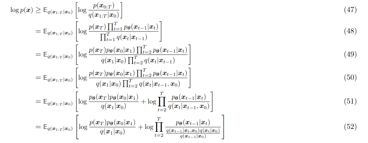
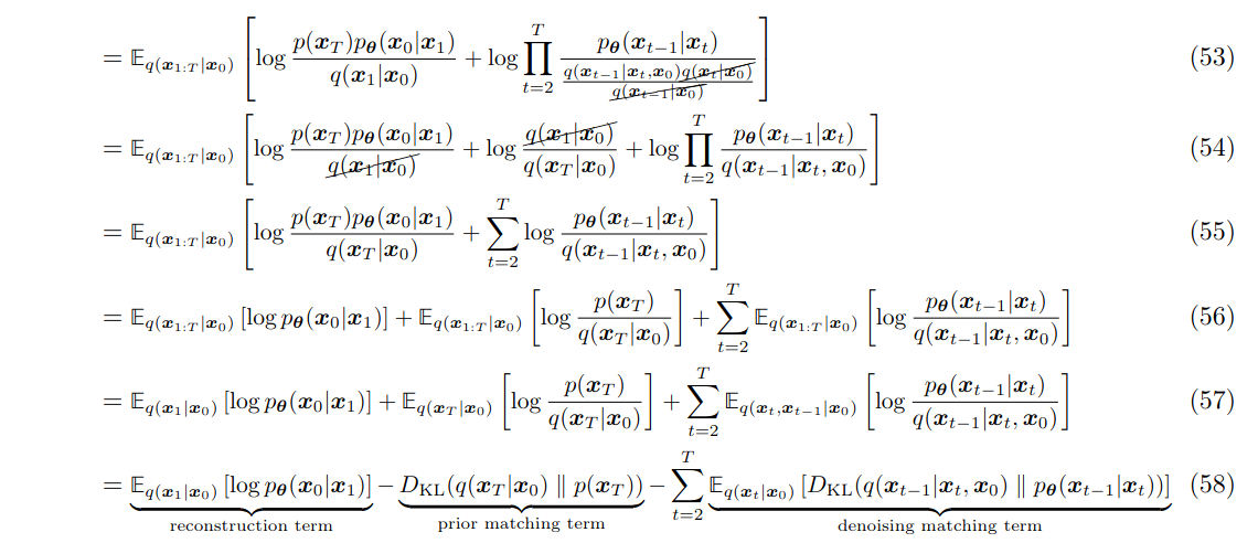
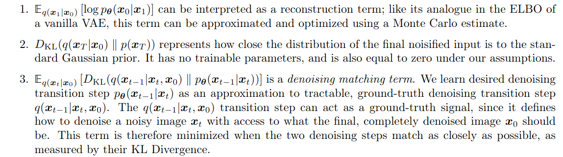
From simple derivation (mainly decomposing 1 into fractional division), we get: $p(x^0)=\int dx^{1…T}q(x^{1…T}|x^0)p(x^T)\prod_{t=1}^T\frac{p(x^{t-1}|x^t)}{q(x^t|x^{t-1})}$. We just need to make this distribution equal to $q(x^0)$. From observation, in the above formula $p(x^T)$ is well-behaved and known, so we can learn $p(x^{t-1}|x^{t})$ through neural networks. We first use cross entropy to get the model optimization objective. To get the following formula, we just need to expand $p(x^0)$ in cross entropy:

\[\begin{align*} L &\geq K= \int dx^{0...T}q(x^{0...T})\log[p(x^T)\prod_{t=1}^T\frac{p(x^{t-1}\|x^t)}{q(x^t\|x^{t-1})}] \\ K &= \sum_{t=1}^T\int dx^{0...T}q(x^{0...T})\log[\frac{p(x^{t-1}\|x^t)}{q(x^t\|x^{t-1})}]+\int dx^Tq(x^T)\log p(x^T) \end{align*}\]

From Jensen’s inequality in integral form and $\log$ being a convex function, we have a lower bound:

\[L \geq K= \int dx^{0...T}q(x^{0...T})\log[p(x^T)\prod_{t=1}^T\frac{p(x^{t-1}\|x^t)}{q(x^t\|x^{t-1})}]\]

Naturally we expand the product in the logarithm:

\[K=\sum_{t=1}^T\int dx^{0...T}q(x^{0...T})\log[\frac{p(x^{t-1}\|x^t)}{q(x^t\|x^{t-1})}]+\int dx^Tq(x^T)\log p(x^T)\]

The first term on the right side of the equation is the exchange of integral and sum, the second term can split* $dx^{0…T}=dx^0dx^1…dx^T$ and then exchange integral order. We denote this term as $-H_p(X^T)=\int dx^Tq(x^T)\log p(x^T)$ which is obviously a cross entropy constant (because it’s well-behaved, i.e., normal). Note that the notation $X^T$ is the random variable itself while $x^T$ is a sample.

Since $\beta$ is small, we can approximately consider $p(x^0|x^1)=q(x^1|x^0)$. Also, since the forward process is Markovian, we can rewrite as:

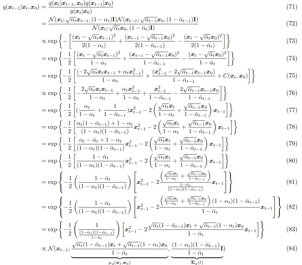
\[K=\sum_{t=2}^T\int dx^{0...T}q(x^{0...T})\log[\frac{p(x^{t-1}\|x^t)}{q(x^t\|x^{t-1}, x^0)}]-H_p(X^T)\]

From Bayes’ formula we have $q(x^t|x^{t-1},x^0)=q(x^{t-1}|x^t, x^0)\frac{q(x^t|x^0)}{q(x^{t-1}|x^0)}$. We rewrite the above formula and extract the product in the logarithm:

\[K=\sum_{t=2}^T\int dx^{0...T}q(x^{0...T})\log[\frac{p(x^{t-1}\|x^t)}{q(x^{t-1}\|x^{t}, x^0)}]+\sum_{t=2}^T\int dx^{0...T}q(x^{0...T})\log[\frac{q(x^{t-1}\|x^0)}{q(x^t\|x^0)}]-H_p(X^T)\]

We expand the differential terms like before and exchange order, then the middle term equals $\sum_{t=2}^T[H_q(X^{t-1}|X^0)-H_q(X^t|X^0)]=H_q(X^T|X^0)-H_q(X^1|X^0)$, which is a number independent of $p$.

Recalling KL divergence: $D_{KL}(q,p)=\int q(x)\log\frac{q(x)}{p(x)}dx=-\int q(x)\log\frac{p(x)}{q(x)}dx$. Using the method of expanding differentials and exchanging, we can rewrite the first term as: $-\sum_{t=2}^T\int dx^0 dx^t q(x^0,x^t)D_{KL}(q(x^{t-1}|x^t,x^0)|p(x^{t-1}|x^t))$. Note that* $dx^{t-1}$ is merged into the divergence, and other differential terms that don’t appear are integrated out. Specifically, we have $q(x^{0…T})=q(x^{t-1}|x^t,x^0)q(x^t,x^0)q(x^{…}|x^t,x^{t-1},x^0)$, so the first term of the product is merged, the second term is retained, and the third term is integrated out.

Therefore, minimizing the divergence through maximum likelihood becomes the optimal solution.

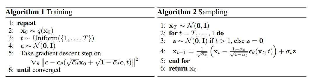
2.2 Implementation

Note that training here is one-step, sampling is the real reverse process. I’ll write the reason in the next few subsections as extended content. One thing to note is that the sampling process here is still sampling from $p(x_{t-1}|x_t, x_0)$, not predicting $x_0$ and then sampling from $p(x_{t-1}|x_0)$. Actually the latter sampling method is exactly the basis of DDIM.

There’s another question: why predict $\epsilon$ instead of the mean? Please see experimental proof:

1. Jonathan Ho, Ajay Jain, and Pieter Abbeel. Denoising diffusion probabilistic models. Advances in Neural Information Processing Systems, 33:6840–6851, 2020.

2. Chitwan Saharia, William Chan, Saurabh Saxena, Lala Li, Jay Whang, Emily Denton, Seyed Kamyar Seyed Ghasemipour, Burcu Karagol Ayan, S Sara Mahdavi, Rapha Gontijo Lopes, et al. Photorealistic text-to-image diffusion models with deep language understanding. arXiv preprint arXiv:2205.11487, 2022

2.2 Another Proof for Reverse

You might wonder why the boundary terms were directly ignored in section 3.1. Here’s a more rigorous derivation:

2.3 Standard DDPM Coefficients

2.4 Simplify Training

You might wonder why training needs to be one-step? Here’s the explanation:

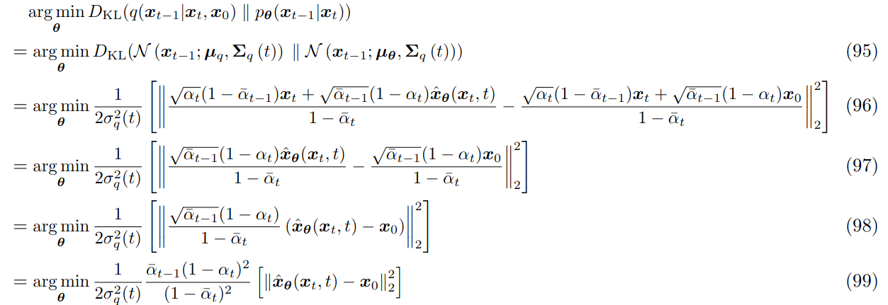
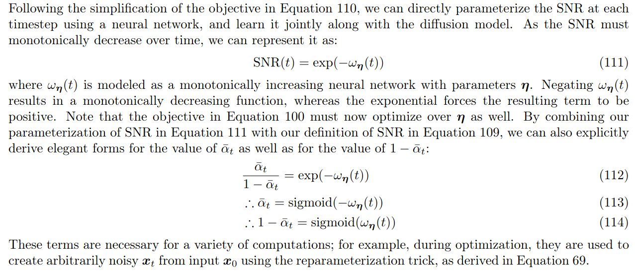
Note that in the second equality, the term on the right side of the minus sign is the prior distribution. Of course, the coefficients here can be transformed as: $\frac{\bar\alpha_{t-1}(1-\alpha_t)^2}{(1-\bar\alpha_t)^2}=(\frac{\bar\alpha_{t-1}}{1-\bar\alpha_{t-1}}-\frac{\bar\alpha_{t}}{1-\bar\alpha_{t}})$. We can introduce the concept of Signal-to-Noise Ratio (SNR) $SNR=\frac{\mu^2}{\sigmasqr}\triangleq\frac{\bar\alpha}{1-\bar\alpha}$, then we have:

\[\frac{\bar\alpha_{t-1}(1-\alpha_t)^2}{(1-\bar\alpha_t)^2}[\parallel \hat x_\theta(x_t,t)-x_0\parallel^2_2]=(SNR(t-1)-SNR(t))[\parallel \hat x_\theta(x_t,t)-x_0\parallel^2_2]\]

2.5 Playing with SNRs

3. DDIMs

In DDPM, we change $\sigma_t=0$ in sampling to get DDIM. Essentially, DDIM theoretically proved that changing such a variance coefficient is still feasible (no additional training needed). For Chinese explanation, please refer to https://kexue.fm/archives/9181

4. Score-based DDPM

4.1 Tweedie’s Formula

https://efron.ckirby.su.domains/papers/2011TweediesFormula.pdf

Theorem. If $z\sim\mathcal{N}(z;\mu_z,\Sigma_z)$ and $\mu_z\sim\pi(\mu_z)$

Then we have $\E[\mu_z|z]=z+\Sigma_z\nabla_z\log p(z)$

Proof. Let $\mathcal{N}(z;\mu_z,\Sigma_z)=p(z|\mu_z)$, we have $L=\int p(z|\mu_z)\pi(\mu_z)d\mu_z$, then

\[\begin{align*} \nabla_zL&=\int \nabla_z\frac{1}{\sqrt{(2\pi)^k\|\Sigma_z\|}}e^{-\frac{1}{2}(z-\mu_z)^T\Sigma_z^{-1}(z-\mu_z)}\pi(\mu_z)d\mu_z \text{ where } k=\text{rank}(\Sigma_z)\\ &= \int p(z\|\mu_z)\Sigma_z^{-1}(\mu_z-z)\pi(\mu_z)d\mu_z \end{align*}\]

Also we have $p(\mu_z|z)=\frac{p(z|\mu_z)\pi(\mu_z)}{p(z)}=\frac{p(z|\mu_z)\pi(\mu_z)}{L}$

\[\begin{align*} \E[\mu_z\|z]&=\int \mu_zp(\mu_z\|z)d\mu_z\\ &=\int(\mu_z-z)p(\mu_z\|z)d\mu_z+\int zp(\mu_z\|z)d\mu_z\\ &= \Sigma_z\frac{\nabla_zL}{L}+z\\ &=z+\Sigma_z\nabla_z\log L \end{align*}\]

4.2 DDPM in Score-based View

In the forward process, using Tweedie’s Formula, note that $x_t\sim\mathcal{N}(x_t;\mu_{x_t},\Sigma_{x_t})$ and $\mu_{x_t}=\sqrt{\bar \alpha_t}X_0\sim\pi(\mu_{x_t})$. Therefore, introducing the probability measure $p_{x_0}$ under $X_0=x_0$, we have the following formula: $\sqrt{\ba_t}x_0=\E[\mu_{x_t}|x_t]=x_t+(1-\ba_t)\nabla_{x_t}\log p_{x_0}(x_t)$

For what we want to learn, substituting the above formula and rearranging to get $x_0$:

\begin{align} \mu_q(x_t,x_0)&=\E [q(x_{t-1}|x_t,x_0)]=\frac{\sqrt{\alpha_t}(1-\ba_{t-1})x_t+\sqrt{\ba_{t-1}}(1-\alpha_t)x_0}{1-\ba_t}
&= \frac{1}{\sqrt{\alpha_t}}x_t+\frac{1-\alpha_t}{\sqrt{\alpha_t}}\nabla_{x_t}\log p_{x_0}(x_t) \end{align}

So from this perspective, DDPM is essentially learning $\nabla_{x_t}\log p_{x_0}(x_t)$ (up to a coefficient). You might ask how this gradient estimation under probability measure $p_{x_0}$ can approximate the entire distribution through Langevin process? Please see Chapter 8.4 of this document.

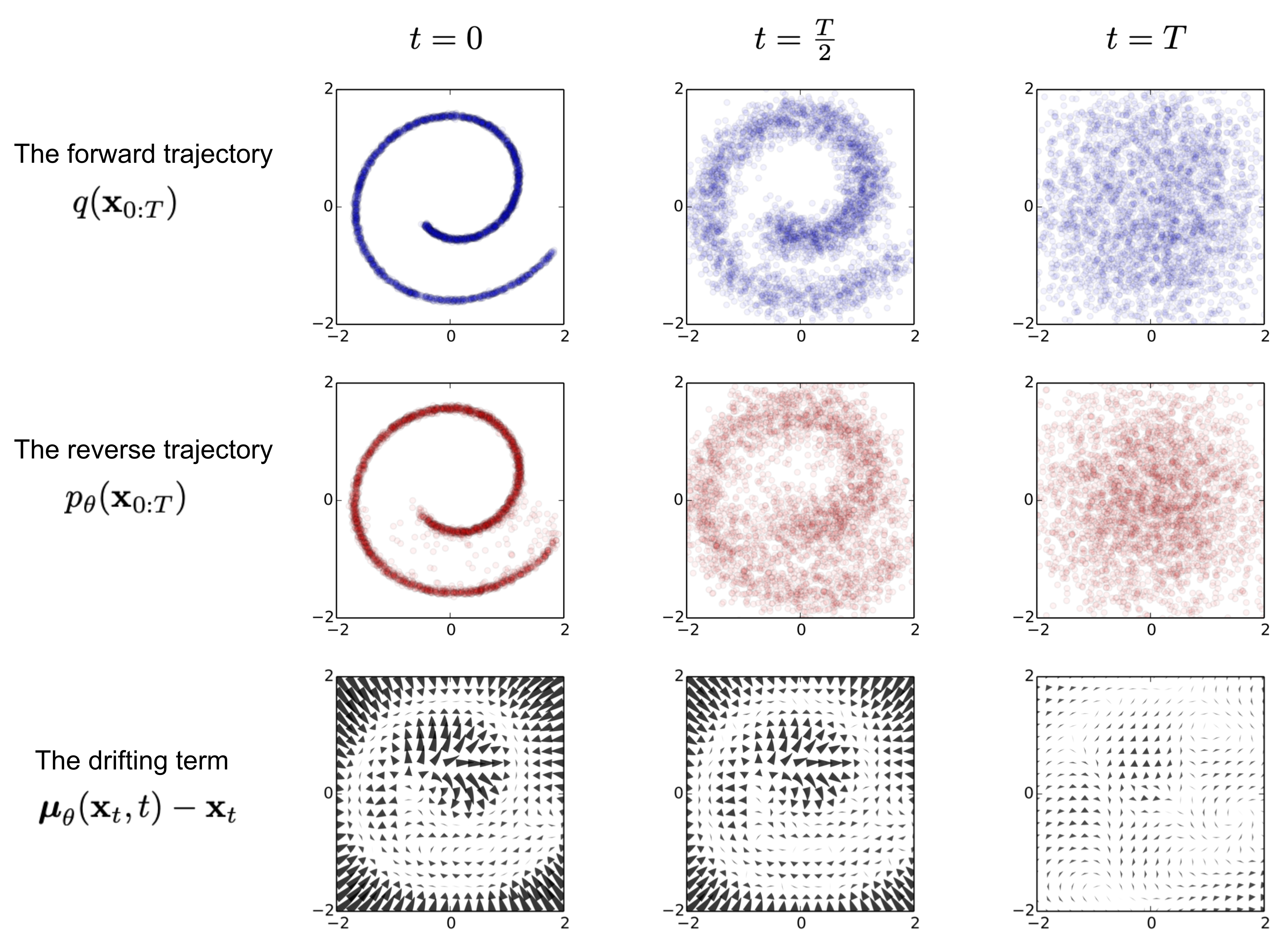
A figure from DDPM’s 2015 paper nicely explains this relationship. You can see that $\mu_\theta(x_t,t)-x_t$ in the figure below shows the appearance of a gradient, which is essentially the embodiment of the formula we derived above. Actually, DDPM is a type of coefficient-hidden Langevin sampling.

5. Guidance DDPM

With the above foundation, I believe this section is easy, so it’s brief

5.1 Classifier Guidance

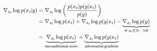
This method requires a pre-trained classifier to provide adversarial gradients, and in the original paper the adversarial gradient is multiplied by a coefficient.

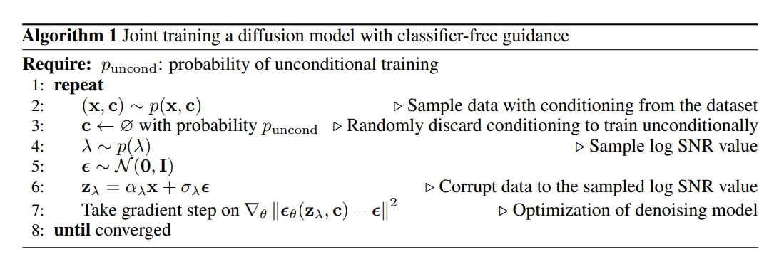
5.2 Classifier-free Guidance

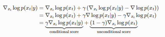
The coefficient control in this method is completed through conditional clipping in the following algorithm.

6. Latent Diffusion Model

With the above foundation, I believe this is easy to grasp: https://www.zhangzhenhu.com/aigc/%E7%A8%B3%E5%AE%9A%E6%89%A9%E6%95%A3%E6%A8%A1%E5%9E%8B.html

7. Score-based SDE Model

Consider a homogeneous differential equation $dX_t=a(X_t,t)dt+b(X_t,t)dW_t$ where $W_t$ is Brownian (Wiener) motion. If we discard the higher-order infinitesimal terms that are extra in increments compared to differentials, and make an informal approximation, we have $\Delta X_t=a(X_t,t)\Delta t+b(X_t,t)\Delta W_t$. We get a unified form of DDPM and DDIM. This is actually a zero-order preserving numerical discretization technique called the Euler-Maruyama method.

More specifically, since Brownian motion has independent stationary increments, we have $\Delta W_t\sim\mathcal{N}(0,\sigma)$, which is the reparameterized random term. When the coefficient of this term becomes 0, we get DDIM, which is the ODE form of diffusion models.

The above is an intuitive explanation. We now rigorously use SDE to represent the diffusion process.

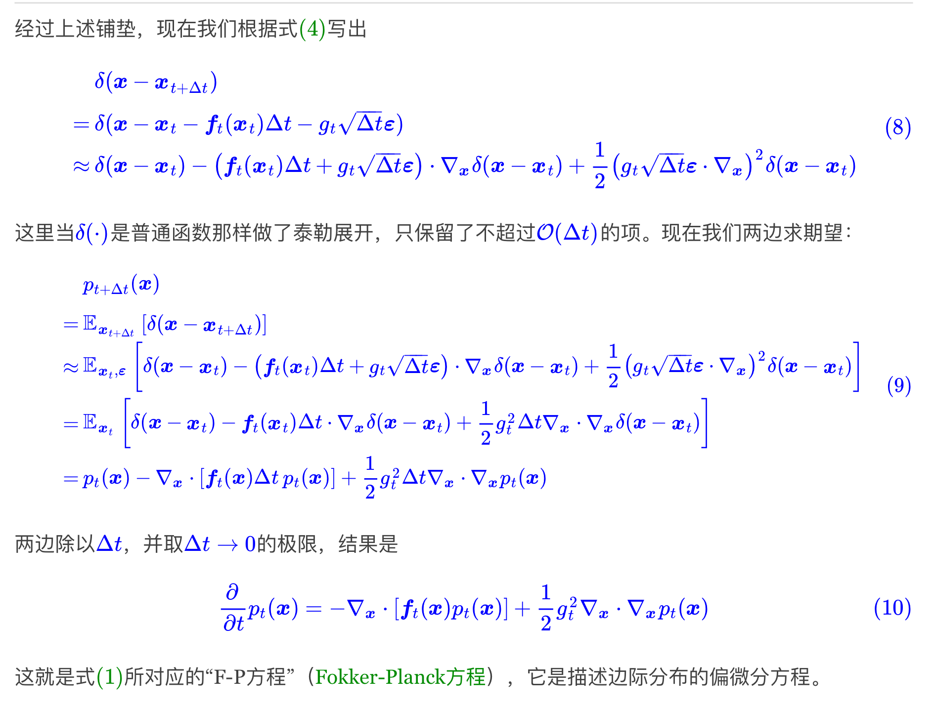
7.1 Fokker-Planck Equation

For a diffusion process $dX_t=\mu(X_t,t)dt+\sigma(X_t,t)dW_t$, let $p(x,t)$ be the density function of the distribution of $X_t$, then we have $\frac{\partial}{\partial t}p(x,t)=-\frac{\partial}{\partial x}[\mu(x,t)p(x,t)]+\frac{\partial^2}{\partial x^2}[D(x,t)p(x,t)]$, where $D(X_t,t)=\frac{\sigmasqr(X_t,t)}{2}$. The high-dimensional case is $\frac{\partial}{\partial t}p(x,t)=-\nabla_x\cdot[\mu(x,t)p(x,t)]+\nabla_x\cdot\nabla_x[D(x,t)p(x,t)]$. For the proof process, please see https://sites.me.ucsb.edu/~moehlis/moehlis_papers/appendix.pdf

For those seeing this equation for the first time, it’s necessary to master the following summation form: $\frac{\partial}{\partial t}p(x,t)=-\sum_{i=1}^N\frac{\partial}{\partial x_i}[\mu_i(x,t) p(x,t)]+\sum_{i=1}^N\sum_{j=1}^N\frac{\partial^2}{\partial x_i\partial x_j}[D_{ij}(x,t)p(x,t)]$ where $D=\frac{1}{2}\sigma\sigma^T$. This points out not to forget that this partial derivative is a scalar. For those unfamiliar with the gradient operator, remember that $\nabla f\neq\nabla\cdot f$. Also for the gradient operator acting on matrices $\nabla\cdot A=(\frac{\partial}{\partial x_1},\frac{\partial}{\partial x_2}…\frac{\partial}{\partial x_N})\times A$ this is matrix multiplication. Also note that $\nabla_x$ acting on vectors is the Jacobian.

Or a simplified proof (using Dirac function i.e. unit impulse function):

7.2 Langevin Dynamics

After having the Fokker-Planck equation, we look for an invariant distribution (considering only one-dimensional case here) $p_\infty(x,t)$ s.t. $\frac{\partial}{\partial t}p_\infty(x,t)=0$, which means $\frac{\partial}{\partial x}[\frac{\partial}{\partial x}(D(x,t)p(x,t))-\mu(x,t)p(x,t)]=\frac{\partial}{\partial x}J=0$, holds for all $x$. Then we have $J=\text{const.}$, that is:

\[\begin{align*} \frac{\partial}{\partial x}D(x,t)p(x,t)&=\mu(x,t)p(x,t)+C \\ \to \frac{\partial}{\partial x}p(x,t)&=\frac{p(x,t)[\mu(x,t)-D_x(x,t)]+C}{D(x,t)} \end{align*}\]

In Langevin dynamics (or diffusion processes in probability theory) $\sigma(X_t,t)=\sqrt{2}\sigma$, where $\sigma$ is a constant (or only depends on $t$ as $\sigma(t)$). This way it’s easy to integrate and get $p_\infty(x,t)\propto \exp(-\frac{\Mu^x(x,t)}{\sigmasqr})$, then we just need to let $\Mu^x(x,t)=-\sigmasqr\log q(x)$ to use stochastic differential equations to sample from target distribution $q(x)$ (here $\Mu$ is uppercase $\mu$, notation meaning the $x$-containing terms of the antiderivative of $\mu$, i.e., $\Mu^x(x,t)=\int\mu(x,t) dx$).

Thus we get $dX_t=-\sigmasqr\nabla_x\log q(x)dt+\sqrt{2}\sigma dW$. Then using the Euler-Maruyama method we get $x_{t+1}=x_t-\sigmasqr\nabla_x\log q(x)\Delta t+\sqrt{2}\sigma \Delta W$. For SGM, by fitting $\nabla_x\log q(x)$ through Score-matching, generation can be performed.

Note that $\sigma$ cannot always be $0$, that is, the forward process $dX_t=\mu(X_t,t)dt+\sigma(X_t,t)dW_t$ of SDE cannot degenerate to $dX_t=\mu(X_t,t)dt$, otherwise it degenerates to $\mu(x,t)p(x,t)=\text{const}$, $dX_t=\mu(x,t)dt$ being a forward ODE. This becomes Flow-based models. If we want $p(x,T)=\mathcal{N}(0,1)$, then we can let $\mu(x,t)=\pi(x)$. Of course it’s definitely not that simple because this is only the one-dimensional case. For high-dimensional cases, I’ll derive it when I find time.

7.3 Inverse Langevin Dynamics

Since it involves the Kolmogorov Reverse Equation, I’ll give it directly. For detailed process, refer to https://ludwigwinkler.github.io/blog/ReverseTimeAnderson/.

For such a process $dX_t=f(X_t,t)dt+g(t)dW$, there’s a reverse process $dX_t=[f(X_t,t)-g^2(t)\nabla_xp(x,t)\vert_{x=X_t, t=t}]dt+g(t)d\bar{W}$, where obviously $dX_t\triangleq X_{t-\Delta t}-X_t$.

Here’s a concise but perhaps not rigorous proof: $dX_t=\lim_{\Delta t\to 0}X_{t+\Delta t}-X_t$, so we consider this increment in the limiting sense can be written as $X_{t+\Delta t}=X_t+f(X_t,t)\Delta t+g(t)\Delta W$, thus we have $p(X_{t+\Delta t}|X_t)=\mathcal{N}(X_t+f(X_t,t)\Delta t,g^2(t)\Delta tI)$, then by Bayes we have $p(X_t|X_{t+\Delta t})=p(X_{t+\Delta t}|X_t)\exp(\log p(X_t)-\log p(X_{t+\Delta t}))$, then through Taylor expansion we can get the above reverse process, refer to https://blog.csdn.net/weixin_44966641/article/details/135541595.

7.4 DDPM in Langevin Dynamics

Recalling the DDPM form $X_t=\sqrt{\ba_t} X_0+\sqrt{1-\ba_t}\epsilon$, $\epsilon\sim\mathcal{N}(0,I)$, it can be written in diffusion form (all $\ba$ below use themselves as replacements). First write as a stochastic process: $X_t=\sqrt{a_t}X_0+\sqrt{1-a_t}\epsilon$, $\epsilon\sim \mathcal{N}(0,1)$. The noising process is: $p(X_t|X_{t-1}=x_{t-1})=\mathcal{N}(\sqrt{1-\beta_t}x_{t-1},\beta_t I)$. We write it in random variable form as $X_t-\sqrt{1-\beta_t}X_{t-1}=\beta_t(W_t-W_{t-1})$. If we view this as the result of Euler-Maruyama, we have $dX_t=(\sqrt{1-\beta_t}-1)X_tdt+\beta_tdW$. Considering inverse Langevin dynamics we have $dX_t=[(\sqrt{1-\beta_t}-1)X_t-\beta_t^2\nabla_xp_t(X_t)]dt+\beta_td\bar{W}$. Continuing to use Euler-Maruyama we get $X_{t-1}=\sqrt{1-\beta_t}X_t-\beta_t^2\nabla_xp_t(X_t)+\beta_t\epsilon$. But since the reverse of DDPM/DDIM is not according to Euler-Maruyama, the coefficients don’t match up, but it’s roughly the same.

But we can return to the previous problem. Since we’ve already derived $\mu_\theta(x_t,x_0)=\frac{1}{\sqrt{\alpha_t}}x_t+\frac{1-\alpha_t}{\sqrt{\alpha_t}}\nabla_{x_t}\log p_{x_0}(x_t)$, we mentioned in DDPM that $x_0=\frac{x_t+(1-\ba_t)\nabla\log p_{x_0} (x_t)}{\sqrt{\ba_t}}=\frac{x_t-\sqrt{1-\ba_t}\epsilon_\theta(x_t,t)}{\sqrt{\ba_t}}$, which means $\epsilon_\theta(x_t,t)=-\sqrt{1-\ba_t}\nabla\log p_{x_0}(x_t)$. The question is where does $x_0$ come from here? In Calvin Luo’s Understanding diffusion models: A unified perspective, this formula is mentioned, but I think he ignored that for $\sqrt{\ba_t}x_0=\E[\mu_{x_t}|x_t]$ to hold, we must have $X_0=x_0$ as a condition, thus directly writing $\nabla\log p_{x_0}(x_t)$ as $\nabla\log p(x_t)$. If it’s really the latter, then DDPM would become a pure Langevin sampling process.

However, this doesn’t actually matter, because we consider the training process of diffusion $\theta=\argmin_\theta\E_{x_0\sim X_0}[\parallel\epsilon-\epsilon_\theta(x_t,t)\parallel]$. For this expectation we can rewrite it as another form that differs only by a coefficient: $\E_{x_0}[\parallel\nabla\log p(x_t|x_0)-s_\theta(x_t,t) \parallel^2]$, where we can view $s_\theta(x_t,t)=-\frac{1}{\sqrt{1-\ba_t}}\epsilon_\theta(x_t,t)$. We naturally hope $s_\theta(x_t,t)=\nabla\log p(x_t)$. Actually, since training uses expectation (even if it comes from Monte Carlo), we expect this expectation operator to enable the model to learn the score, not the conditional score. Actually, consider this formula:

$\E_{x_0}[\parallel\nabla\log p(x_t)-s_\theta(x_t,t) \parallel]^2-\E_{x_0}[\parallel\nabla\log p(x_t|x_0)-s_\theta(x_t,t) \parallel]^2$

It equals a constant independent of $\theta$. So naturally when we minimize loss, the two are equivalent. For detailed proof refer to https://spaces.ac.cn/archives/9509

I’ll give another perspective. We can intuitively think of $\epsilon_\theta:x_t\mapsto x_0$. We denote this function as $f(x_t)$, then $\epsilon_\theta(x_t,t)=-\sqrt{1-\ba_t}\nabla\log p_{f(x_t)}(x_t)$. We can get the following formula: $f(x_t)=\frac{x_t-\sqrt{1-\ba_t}\epsilon_\theta(x_t,t)}{\sqrt{\ba_t}}$. We can easily rewrite the forward SDE process of DDPM:

$X_{\tau}=\frac{x_t-\sqrt{1-\ba_t}\epsilon_\theta(x_t,t)}{\sqrt{\ba_t}}+\int_0^\tau g(X_\tau,\tau)d\tau+\int_0^\tau\sigma(\tau)dW_\tau$

That is, for the forward process, since $X_0=x_0$ doesn’t change the Markov property, the differential form of the equation remains unchanged, but the integral initial value will collapse to a determined point, which is $x_0=f(x_t)$. For the reverse process, since most likely $f(x_t)\neq f(\hx_{t-1})$, where $\hx_{t-1}$ is sampled by the model according to $\epsilon(x_t,t)$, even if we consider the ODE process $dX_\tau=[f(X_\tau,\tau)-g(\tau)^2\nabla_{x_\tau}\log p_{x_0}(x_\tau)]dt$, we can’t guarantee this ODE will finally lead to $x_0$. Thus the reverse process is probabilistic Langevin sampling, but in any case cannot be a reverse ODE on a single “trajectory”. If we define a “diffusion trajectory” $w(x_0)={X_t|X_0=x_0:t\ge0}$, then it’s equivalent to the model repeatedly switching diffusion trajectories regardless (meaning even if $\sigma=0$), and performing one step of reverse ODE (SDE) on each trajectory. In some sense, this makes fast sampling in the reverse direction of DDPM difficult.

*In all the above descriptions $p(x_t)=p_t(x_t)=p(x_t,t)=p(x,t)=p_t(x)$, while $p_{x_0}(x_t)=p(x_t|x_0)=p(x,t|x_0)…$

*Update: After research, I found that the perspective I proposed is an important problem. Actually, methods to solve diffusion trajectory switching have been proposed, see https://arxiv.org/pdf/2311.01223, which is DDCM — Consistency Diffusion Model.

8. SDE, ODE and All the Equations

After Chapters 1-8, we already have a preliminary understanding of diffusion theory. In this chapter, we’ll systematically organize some other diffusion concepts around this paper: https://arxiv.org/pdf/2011.13456, including improvements proposed in this paper. This will be a solid establishment of the theoretical foundation of the previous text, and also a preparation for the Consistency model proposed in the next chapter.

8.1 Variance Preserving SDE

For DDPM, DDIM and other series models, they all have similar formulas like: $x_t|x_0\sim\mathcal{N}(\sqrt{\ba_t}x_0,\sqrt{1-\ba_t}I)$. It’s not hard to see this is a weighted average of $x_0$ and $\mathcal{N}(0,I)$, with the sum of squared weights being 1. Therefore $\text{Var}(X_t)= \ba_tV_d+(1-\ba_t)I$, where $V_d$ is the dataset variance. So the variance is controllable and converges to $I$, making this process a Variance Preserving SDE. For the recurrence formula $x_{t+1}=\sqrt{1-\beta_{t+1}}x_t+\beta_{t+1}z$, we’ve tried to explain such processes using the Euler method to derive SDE, and now we’ll more precisely derive the SDE formula for such processes:

Consider a sequence ${\beta_t}_{t=1}^N$. In the sense of $N\to\infty$, we can have a continuous function $\beta(t), t\in[0,1]$, s.t. $\beta(\frac{i}{N})=\beta_i$ to represent such a coefficient. The same applies to $x_t$. Then we have:

$x(t+\Delta t)=\sqrt{1-\beta(t+\Delta t)\Delta t}x(t)+\sqrt{\beta(t+\Delta t)}z(t)\approx x(t)-\frac{1}{2}\beta(t)\Delta tx(t)+\sqrt{\beta(t)\Delta t}z(t)$

Therefore we get $dx=-\frac{1}{2}\beta(t)xdt+\sqrt{\beta(t)}dw$.

8.2 Variance Exploding SDE

Another class of diffusion models is SMLD models, which perform the forward process as follows: $x_t=x_{t-1}+\sqrt{\sigmasqr_t-\sigmasqr_{t-1}}z_{t-1}$. We can see that we have $\text{Var}(X_t)= V_d+\sigma_t^2I$, hence called Variance Exploding SDE. Then under the same function defined by the sequence ${\sigma_i}_{i=1}^N$, obviously we have the corresponding SDE:

$x(t+\Delta t)\approx x(t)+\sqrt{\frac{d[\sigmasqr(t)]}{dt}\Delta t}z(t)$

$dx=\sqrt{\frac{d[\sigmasqr(t)]}{dt}}dw$

*Here we just need to view $\sqrt{\Delta t}$ as multiplied with $z(t)$.

TO BE COMPLETED

9. Consistency Models

Dr. Song Yang proposed the DDCM model in 2023 to solve the multi-step sampling problem required by diffusion. Its core idea is to learn a “consistency model” to make the reverse diffusion trajectory unique. For the original paper, see: https://arxiv.org/pdf/2303.01469

9.1 Diffusion ODE Model

We proposed the so-called diffusion trajectory problem in Chapter 8.4. If we further simplify the problem and consider the following ODE diffusion (which can be seen as deterministic sampling SDE):

Forward process: $dX_t=\mu(X_t,t)dt+\sigma(t)dW$

Reverse process: $dX_t=[\mu(X_t,t)-\frac{1}{2}\sigma(t)^2\nabla_{x_t}\log p(x_t)]dt$

We can see that here we just remove the random term of Brownian motion. It can also be seen as a deterministic reverse trajectory.

We consider the following VE (Variance Exploding) setting: $\mu(X_t,t)=0, \sigma(t)=\sqrt{2t}$. Then the forward process has $X_t=X_0+\mathcal{N}(0,I\int_0^t \sqrt{2t}dt)=X_0+\mathcal{N}(0,t^2I)$, then $p_t(X)=p_0(X)\times \mathcal{N}(0,t^2I)$ where the multiplication sign is convolution. This result is obvious for those who have taken probability theory. Also approximately we have $\pi(x)=\mathcal{N}(0,T^2I)$. Then we can get $dX_t=-ts_\theta(x_t,t)$. We can sample a sample in about 80 steps using reverse ODE solvers. However, this is still not fast enough, which is why we need Consistency Model. Although such a reverse ODE is not what we want, the reverse ODE has a very good property, namely “Consistency”, that is, for a determined $X_t$, its reverse trajectory is determined. Such determinism is exactly what we want. Therefore, to quickly get this deterministic trajectory sampling, we consider parameterizing the reverse ODE process + score function, using neural networks to learn.

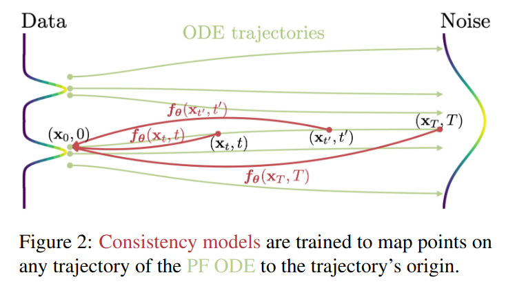
9.2 Consistency Model

So our goal becomes finding a $f_\theta(x,t)$ that satisfies the following equation:

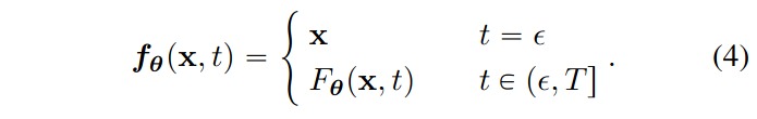
Also for the ODE process we have $f_\theta(x,t)=f_\theta(x’,t’)$ where $x’$ is a point on the path obtained by $x$ through the reverse ODE process. $\epsilon$ is chosen to be a small quantity instead of $0$ for numerical stability. $F_\theta(x,t)$ is a free-form neural network that only needs to output the same shape as the input $x$.

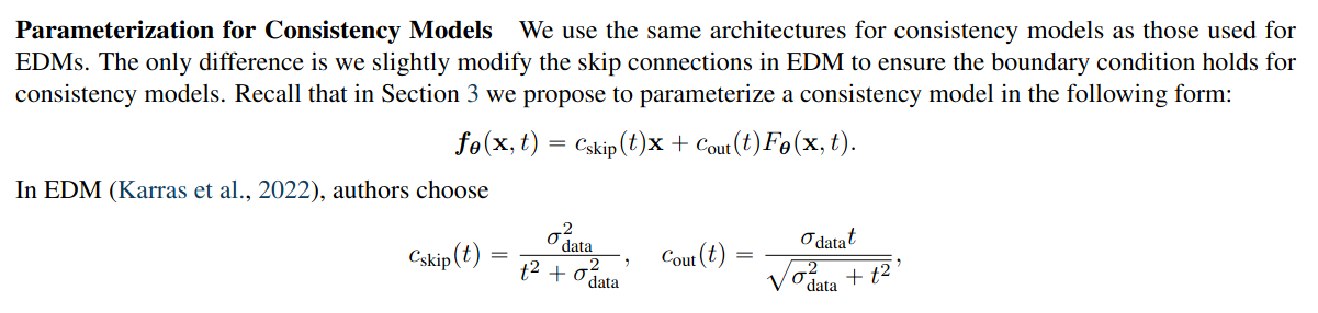
Then we can parameterize it as: $f_\theta(x,t)=c_{\text{skip}}(t)x+c_{\text{out}}(t)F_\theta(x,t)$ where when $t=\epsilon$ we have $c_{\text{skip}}=1, c_{\text{out}}(t)=0$ and these two functions are differentiable. This successfully constructs a parameterized (neural network-based) reverse consistency model. Then we just need to train according to the above constraints. There’s a way to distill from already trained score functions as follows:

The technique of using two networks and EMA updates is a common technique used by many models like DINO. Here’s an explanation of the step $\hx_{t_n}^\phi\leftarrow x_{t_{n+1}}+(t_n-t_{n+1})\Phi(x_{t_{n+1}},t_{n+1};\phi)$. This is actually a single-step ODE solver iteration process. For example, if we consider the simplest Euler solving, we have $\hx_{t_n}^\phi\leftarrow x_{t_{n+1}}+(t_n-t_{n+1})t_{n+1}s_\phi(x_{t_{n+1}},t)$.

Of course, the original paper also proposed integrated training methods that don’t require such distillation, and proved that $\nabla_{x_{t}} \log p_t(x_t)=-\E_{x\sim p_0(x_0)}[\frac{x_t-x}{t^2}|x_t]$, thus using this to replace already trained models for training. For details, see the original paper. It’s also necessary to point out that several key functions take the following values (proof in Chapter 9):

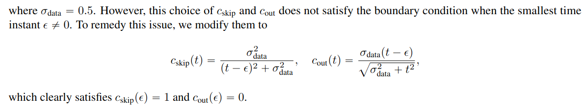
9.3 SSS Consistency Model

In Consistency Model, Song Yang proposed general CM formulation. However, the trickiest thing is actually the choice of $c_{\text{skip}}, c_{\text{out}}$ functions, which extremely requires mathematical derivation. Therefore, on top of this, Song Yang et al. simplified CM while optimizing stability, etc., obtaining SIMPLIFYING, STABILIZING & SCALING CONTINUOUS-TIME CONSISTENCY MODELS: https://arxiv.org/pdf/2410.11081v1

10. Discussion

[This section appears to be a placeholder for future discussion]